Find the relavant RAVs using metadata

Abstract

Setup

Load packages

if (!"GenomicSuperSignaturePaper" %in% installed.packages())
    devtools::install_github("shbrief/GenomicSuperSignaturePaper")

## Load packages
suppressPackageStartupMessages({
  library(GenomicSuperSignature)
  library(GenomicSuperSignaturePaper)
  library(ggplot2)
  library(ggpubr)
  library(dplyr)
  library(Biobase)
})
## Warning: package 'GenomicSuperSignature' was built under R version 4.1.3

RAVmodel

RAVmodel <- getModel("C2", load=TRUE)

RAVmodel
## class: PCAGenomicSignatures 
## dim: 13934 4764 
## metadata(8): cluster size ... version geneSets
## assays(1): RAVindex
## rownames(13934): CASKIN1 DDX3Y ... CTC-457E21.9 AC007966.1
## rowData names(0):
## colnames(4764): RAV1 RAV2 ... RAV4763 RAV4764
## colData names(4): RAV studies silhouetteWidth gsea
## trainingData(2): PCAsummary MeSH
## trainingData names(536): DRP000987 SRP059172 ... SRP164913 SRP188526

version(RAVmodel)
## [1] "1.1.1"

CRC validation datasets

load("data/eSets/setNames.RData")

eSets_new data is available upon request.

## Load validation samples
for (set in setNames) {
  load(paste0("data/eSets_new/", set, '.RData'))
}

Get phenotype data

Combine all the phenotype data from CRC validation datasets.

## phenotype tables combined
pdata_df <- setNames %>% lapply(function(set) {
  eSet <- get(set)
  pdata <- pData(eSet)
  eSet_tmp <- eSet[, pdata$sample_type %in% "tumor"]
  pdata_tmp <- pData(eSet_tmp)
  
  ind_rm <- grep("CRIS_", colnames(pdata_tmp))
  if (length(ind_rm) != 0) {pdata_tmp <- pdata_tmp[,-ind_rm]}
  pdata_tmp$study <- set  # add 'study' column
  
  return(pdata_tmp)
}) %>% Reduce('rbind', .)

Get expression data

Combine all the expression profiles from CRC validation datasets and subset it with the common genes among them.

## common genes between all validation datasets
all_genes <- list()
for (set in setNames) {
  eSet <- get(set)
  exprs <- exprs(eSet) %>% rmNaInf
  all_genes[[set]] <- rownames(exprs)
}
cg <- Reduce(intersect, all_genes)

## expression matrix combined
exprs_df <- setNames %>% lapply(function(set) {
  eSet <- get(set)
  pdata <- pData(eSet)
  eSet_tmp <- eSet[cg, pdata$sample_type %in% "tumor"]
  exprs_tmp <- exprs(eSet_tmp) %>% rmNaInf
  exprs_tmp <- apply(exprs_tmp, 1, function(x) x - mean(x)) %>% t
  return(exprs_tmp)  
}) %>% Reduce('cbind', .)   # 8219 genes x 3567 samples

Calculate sample scores

Calculate sample scores and combine them with the phenotype data.

sampleScore <- calculateScore(exprs_df, RAVmodel)
data_all <- cbind(sampleScore, pdata_df)

Metadata-based search

In this section, we identified the desired RAVs using metadata. As an example of discrete, multivariate metadata, we used four CMS subtypes.

Multivariable

ANOVA

f.stat.all <- sapply(seq_len(ncol(RAVmodel)), function(x) {
  res.aov <- aov(data_all[,x] ~ data_all$cms_label_SSP)
  f.stat <- summary(res.aov)[[1]][1,4]   # extract F-statistics from ANOVA 
  return(f.stat)
})

names(f.stat.all) <- paste0("RAV", seq_len(ncol(RAVmodel)))
head(f.stat.all[order(f.stat.all, decreasing = TRUE)])
##    RAV834    RAV833    RAV861    RAV188   RAV2432    RAV579 
## 1216.5445  834.3780  742.6224  709.8732  656.5008  642.1502

Kruskal-Wallis Rank Sum Test

Based on the Q-Q plot below, the normality assumption is not met.

res.aov <- aov(data_all[,"RAV834"] ~ data_all[,"cms_label_SSP"])
plot(res.aov, 2)

Try Kruskal-Wallis Rank Sum Test

# Kruskal-Wallis Rank Sum Test : a non-parametric alternative to one-way ANOVA, 
# when normality assumption is not met
kw.chi.sqr <- sapply(seq_len(ncol(RAVmodel)), function(x) {
  kw.test <- kruskal.test(data_all[,x] ~ data_all$cms_label_SSP)
  kw.stat <- kw.test$statistic
  return(kw.stat)
})

names(kw.chi.sqr) <- paste0("RAV", seq_len(ncol(RAVmodel)))
head(kw.chi.sqr[order(kw.chi.sqr, decreasing = TRUE)])
##   RAV834   RAV833   RAV188   RAV579   RAV657  RAV1957 
## 2146.136 1831.683 1829.326 1775.702 1750.150 1693.344

Binary variables

We ran t.test between the four clinical variables and all sample scores. The test results were ordered based on p-value and the top 6 of them are printed. Both MSI and tumor location are explained best with RAV834 while tumor grade and stage seem to be more closely associated with RAV596 and RAV3290, respectively.

MSI

Microsatellite instability

##       RAV834      RAV2013      RAV3599       RAV420      RAV2012       RAV517 
## 3.587747e-99 6.819382e-83 2.164587e-75 9.580321e-61 4.124044e-57 6.586642e-56

Location

Tumor location

##       RAV834      RAV4350      RAV2096      RAV2746      RAV2012      RAV2116 
## 5.224891e-18 4.082548e-14 5.568131e-14 1.420074e-13 1.894671e-13 3.407322e-13

Grade

##       RAV596      RAV2760      RAV1059      RAV1761      RAV3704      RAV3940 
## 5.475896e-11 1.726620e-07 2.198328e-07 8.452389e-07 1.636694e-06 4.207970e-06

Stage

##      RAV3290      RAV2528       RAV234      RAV3264       RAV911       RAV766 
## 6.804255e-15 1.424937e-14 2.557679e-12 4.903492e-12 6.276130e-12 6.996570e-12

Subtyping with RAVs

Score plot

Top two RAVs, RAV834 and RAV833, are identified from both ANOVA and Kruskal-Wallis Rank Sum Test. Below plot shows how these two RAVs are differentiating 18 CRC datasets. More related analyses are done in here.

sampleScore1 <- 834
sampleScore2 <- 833
df.results <- data_all
source("R/Fig4A_plotting.R", print.eval = TRUE)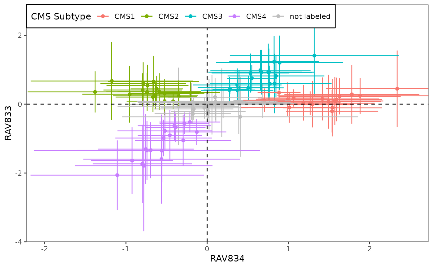

Mean comparing methods

We further quantified how RAV834 separates four CMS subtypes using different mean comparing methods.

t.test for a few pairs

my_comparisons <- list(c("CMS1", "CMS2"),c("CMS1", "CMS3"),c("CMS1", "CMS4"))
ggboxplot(data_all, x = "cms_label_SSP", y = "RAV834", fill = "cms_label_SSP") +
  stat_compare_means(comparisons = my_comparisons, 
                     method = "t.test", aes(label = ..p.adj..))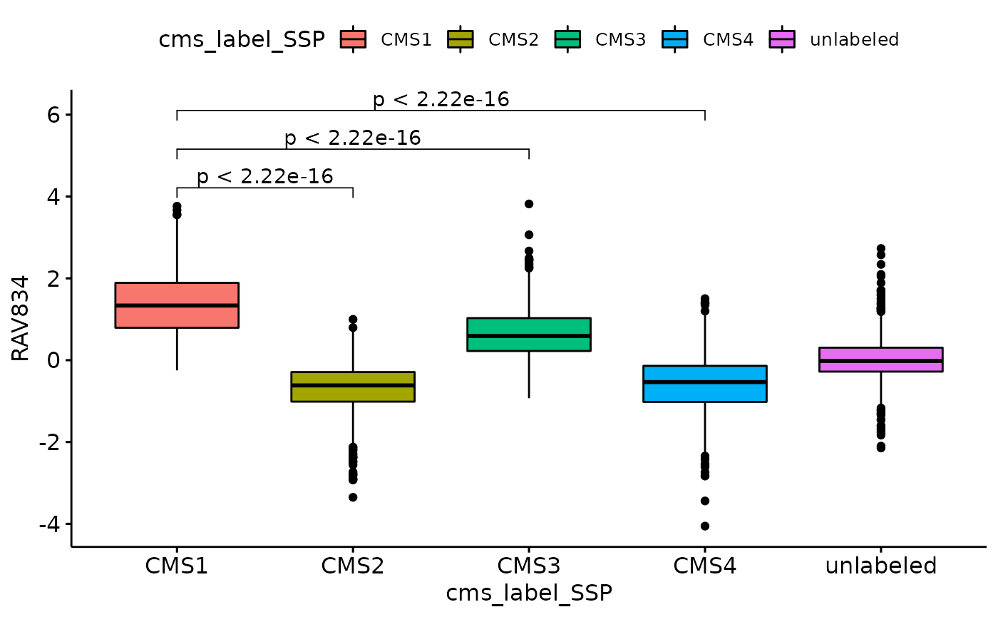

ANOVA

ggboxplot(data_all, x = "cms_label_SSP", y = "RAV834", fill = "cms_label_SSP") +
  stat_compare_means(method = "anova", label.y = 7) # Add global p-value

Kruskal-Wallis Rank Sum Test

ggboxplot(data_all, x = "cms_label_SSP", y = "RAV834", fill = "cms_label_SSP") +
  stat_compare_means(method = 'kruskal.test', label.y = 7) # Add global p-value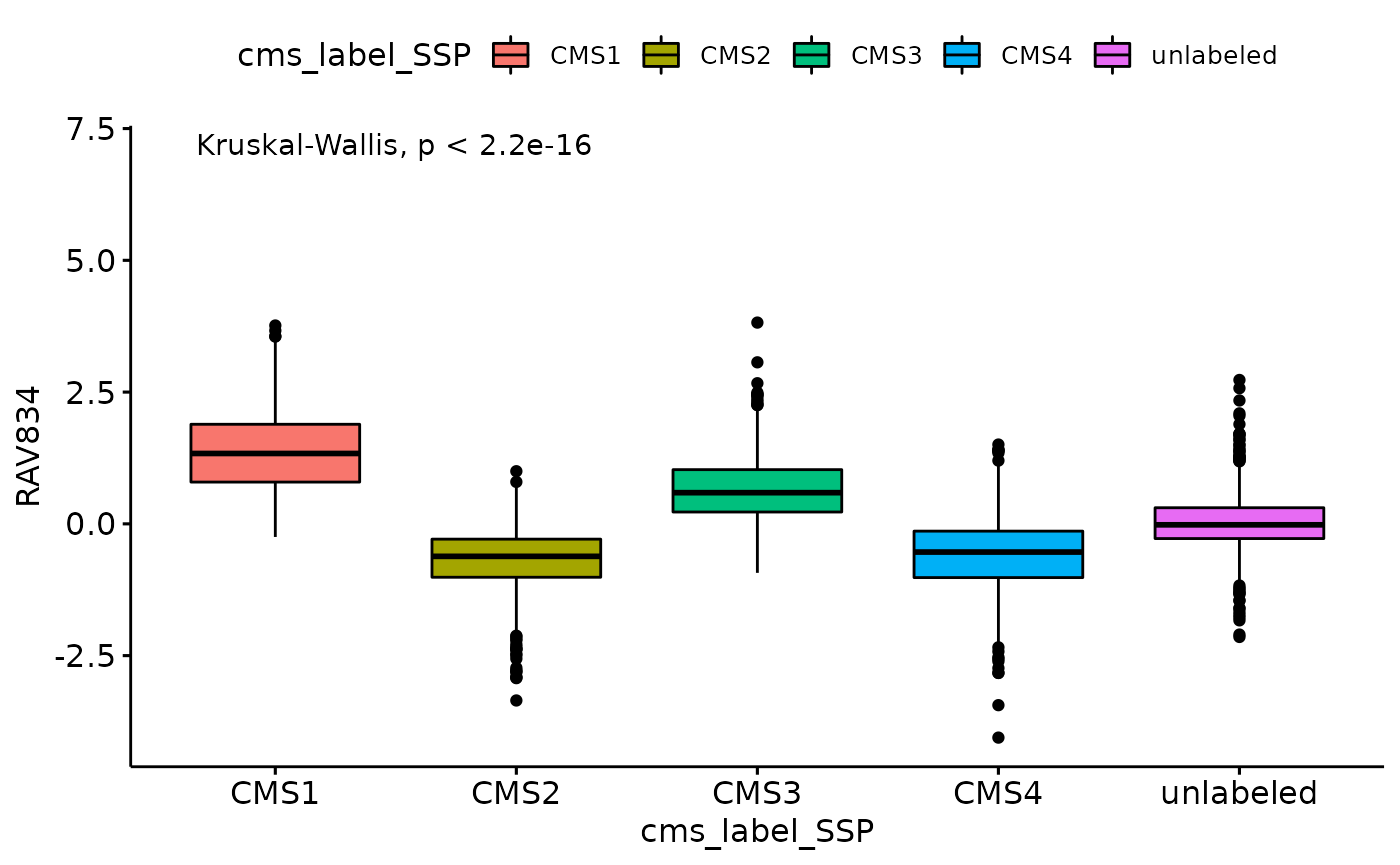

Session Info

sessionInfo()
## R version 4.1.2 (2021-11-01)
## Platform: x86_64-pc-linux-gnu (64-bit)
## Running under: Ubuntu 20.04.3 LTS
## 
## Matrix products: default
## BLAS/LAPACK: /usr/lib/x86_64-linux-gnu/openblas-pthread/libopenblasp-r0.3.8.so
## 
## locale:
##  [1] LC_CTYPE=en_US.UTF-8       LC_NUMERIC=C              
##  [3] LC_TIME=en_US.UTF-8        LC_COLLATE=en_US.UTF-8    
##  [5] LC_MONETARY=en_US.UTF-8    LC_MESSAGES=en_US.UTF-8   
##  [7] LC_PAPER=en_US.UTF-8       LC_NAME=C                 
##  [9] LC_ADDRESS=C               LC_TELEPHONE=C            
## [11] LC_MEASUREMENT=en_US.UTF-8 LC_IDENTIFICATION=C       
## 
## attached base packages:
## [1] stats4    stats     graphics  grDevices utils     datasets  methods  
## [8] base     
## 
## other attached packages:
##  [1] dplyr_1.0.8                      ggpubr_0.4.0                    
##  [3] ggplot2_3.3.5                    GenomicSuperSignaturePaper_1.1.1
##  [5] GenomicSuperSignature_1.3.6      SummarizedExperiment_1.24.0     
##  [7] Biobase_2.54.0                   GenomicRanges_1.46.1            
##  [9] GenomeInfoDb_1.30.1              IRanges_2.28.0                  
## [11] S4Vectors_0.32.3                 BiocGenerics_0.40.0             
## [13] MatrixGenerics_1.6.0             matrixStats_0.61.0              
## [15] BiocStyle_2.22.0                
## 
## loaded via a namespace (and not attached):
##  [1] bitops_1.0-7           fs_1.5.2               bit64_4.0.5           
##  [4] filelock_1.0.2         httr_1.4.2             doParallel_1.0.17     
##  [7] RColorBrewer_1.1-2     rprojroot_2.0.2        tools_4.1.2           
## [10] backports_1.4.1        bslib_0.3.1            utf8_1.2.2            
## [13] R6_2.5.1               DBI_1.1.2              colorspace_2.0-3      
## [16] GetoptLong_1.0.5       withr_2.5.0            tidyselect_1.1.2      
## [19] curl_4.3.2             bit_4.0.4              compiler_4.1.2        
## [22] textshaping_0.3.6      cli_3.2.0              desc_1.4.1            
## [25] DelayedArray_0.20.0    labeling_0.4.2         bookdown_0.25         
## [28] sass_0.4.0             scales_1.1.1           rappdirs_0.3.3        
## [31] pkgdown_2.0.2          systemfonts_1.0.4      stringr_1.4.0         
## [34] digest_0.6.29          rmarkdown_2.13         XVector_0.34.0        
## [37] pkgconfig_2.0.3        htmltools_0.5.2        highr_0.9             
## [40] dbplyr_2.1.1           fastmap_1.1.0          rlang_1.0.2           
## [43] GlobalOptions_0.1.2    RSQLite_2.2.10         farver_2.1.0          
## [46] shape_1.4.6            jquerylib_0.1.4        generics_0.1.2        
## [49] jsonlite_1.8.0         car_3.0-12             RCurl_1.98-1.6        
## [52] magrittr_2.0.2         GenomeInfoDbData_1.2.7 Matrix_1.4-0          
## [55] Rcpp_1.0.8.3           munsell_0.5.0          fansi_1.0.2           
## [58] abind_1.4-5            lifecycle_1.0.1        stringi_1.7.6         
## [61] yaml_2.3.5             carData_3.0-5          zlibbioc_1.40.0       
## [64] BiocFileCache_2.2.1    blob_1.2.2             grid_4.1.2            
## [67] parallel_4.1.2         crayon_1.5.0           lattice_0.20-45       
## [70] circlize_0.4.14        knitr_1.37             ComplexHeatmap_2.10.0 
## [73] pillar_1.7.0           rjson_0.2.21           ggsignif_0.6.3        
## [76] codetools_0.2-18       glue_1.6.2             evaluate_0.15         
## [79] BiocManager_1.30.16    png_0.1-7              vctrs_0.3.8           
## [82] foreach_1.5.2          gtable_0.3.0           purrr_0.3.4           
## [85] tidyr_1.2.0            clue_0.3-60            assertthat_0.2.1      
## [88] cachem_1.0.6           xfun_0.30              broom_0.7.12          
## [91] rstatix_0.7.0          ragg_1.2.2             tibble_3.1.6          
## [94] iterators_1.0.14       memoise_2.0.1          cluster_2.1.2         
## [97] ellipsis_0.3.2

Sehyun Oh

2022-03-24

Setup

Load packages

RAVmodel

CRC validation datasets

Get phenotype data

Get expression data

Calculate sample scores

Metadata-based search

Multivariable

ANOVA

Kruskal-Wallis Rank Sum Test

Binary variables

MSI

Location

Grade

Stage

Subtyping with RAVs

Score plot

Mean comparing methods

t.test for a few pairs

ANOVA

Kruskal-Wallis Rank Sum Test

Session Info