Find the optimum number of clusters for hierarchical clustering

Abstract

Preparae negative controls

Build negative controls

We used the negative-control dataset to explore the optimum number of clusters for hierarchical clustering. Negative-control dataset was built using the below script.

## Do not run this script without checking it first!!
source("neg_controls.R")

This script runs the following processes:

Generate 50 synthetic datasets:
–> Each dataset contains 50 random samples from 44,890 samples (with replacement).
–> Scramble genes in each dataset by random selection without replacement and add random value between -0.1 and 0.1
Row-normalize synthetic datasets
PCA on synthetic datasets
–> saved as bootstrap_PCs_rowNorm_Neg.rds
Combine top 20 PCs from traning datasets and PC1s from synthetic datasets
–> saved as all_{#neg}.rds
Calculate distance matrix and hcut for each combined dataset
–> saved as res_dist_{#neg}.rds and res_hclust_{#neg}.rds
Evaluate how the negative controls were separated
–> saved as evals_{#neg}.rds and eval_summary_{#neg}.rds

Validate negative controls

Below is the summary of the distance matrix of 10,720 PCs (top 20 PCs from 536 studies).

summary(res_dist)
##    Min. 1st Qu.  Median    Mean 3rd Qu.    Max. 
## 0.01688 0.98783 1.00000 0.99999 1.01217 1.97482

We create a synthetic dataset whose distance ranges median or higher of the actual 536 training dataset. Below is the distance matrix of the 50 negative controls generated from the neg_controls.R script. Distance ranges roughly between 1st and 3rd quarters of training dataset’s distance distribution.

summary(res.dist.neg)
##    Min. 1st Qu.  Median    Mean 3rd Qu.    Max. 
##  0.9680  0.9937  1.0000  0.9999  1.0054  1.0317

We plot the heatmap of distance matrix using the different number of negative controls (PC1s from synthetic datasets). They are different within the range we want to separate.

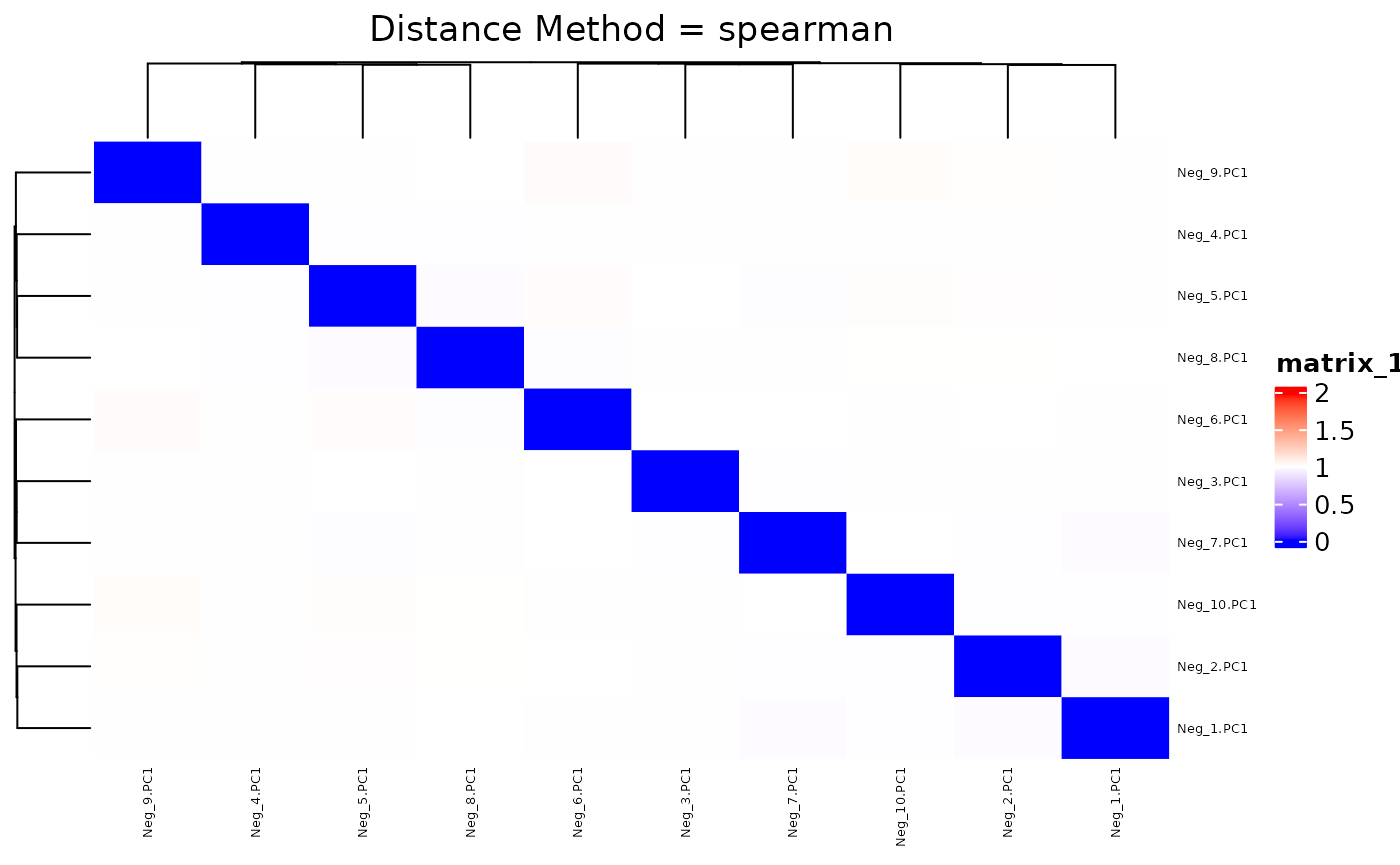
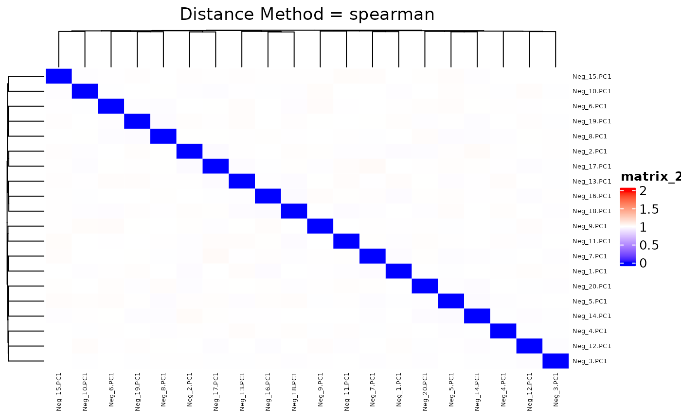
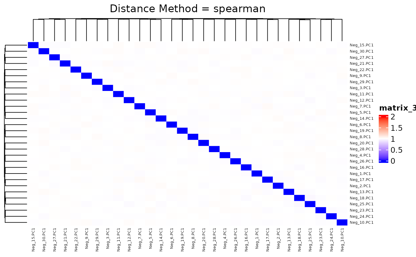
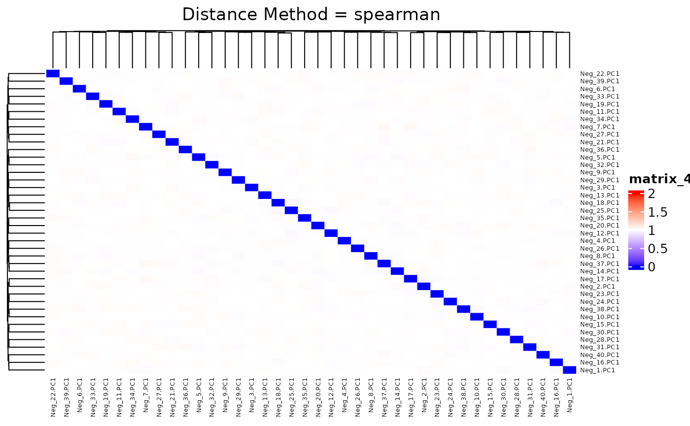
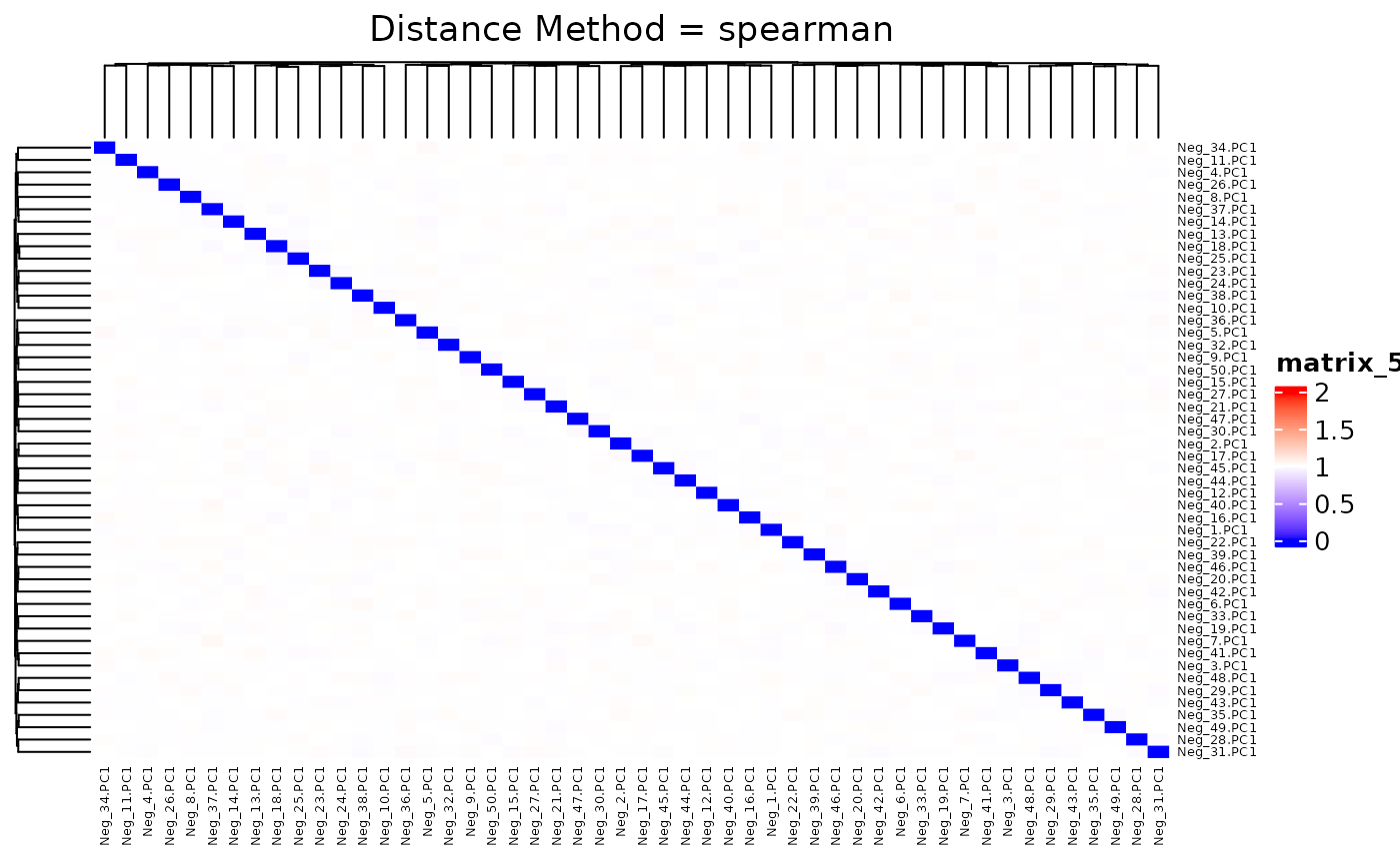
## agg_png 
##       2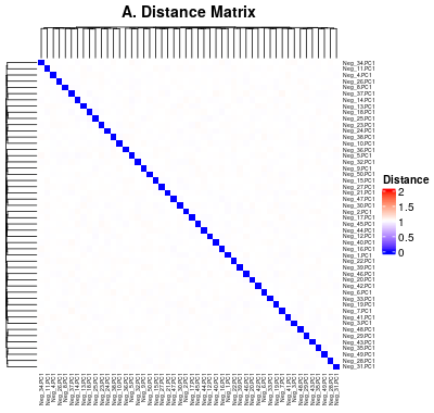

Optimum number of clusters

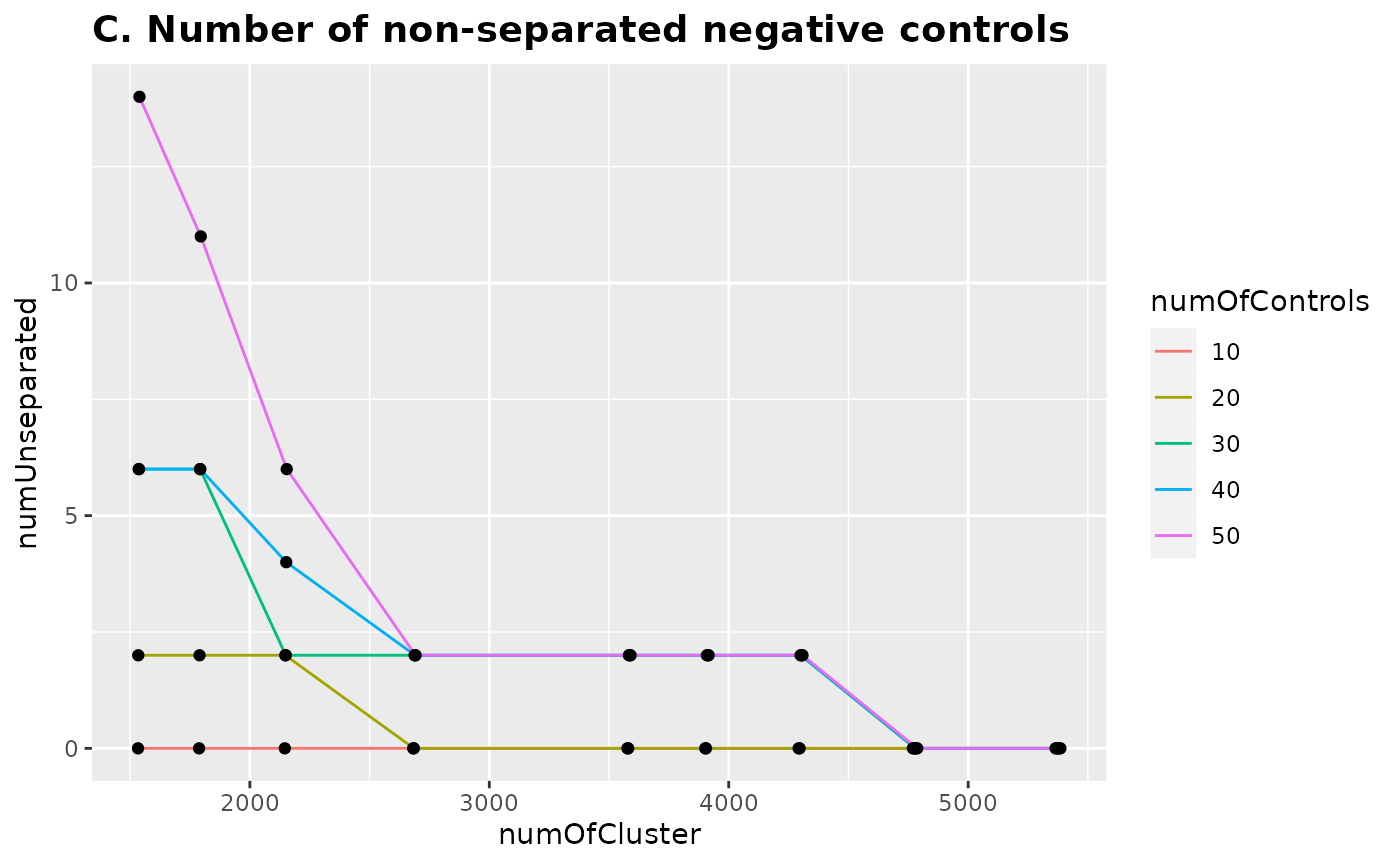
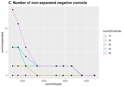
Next we combined top 20 PCs of training datasets and PC1s from the varying numbers of negative controls (10, 20, 30, 40, and 50) and performed hierarchical clustering with the different numbers of clusters. Number of clusters was the rounds of the number of PCs divided by 9 different numbers (d = 7, 6, 5, 4, 3, 2.75, 2.5, 2.25, and 2).

Proportion of the separated

This plot shows the proportion of the negative controls that are separated with the different numbers of clusters. For all five different numbers of negative controls, more than 90% of them were separated when d = 4 and 100% of them were separated when d = 2.25.

## agg_png 
##       2

Number of the non-separated

This plot shows the actual number of negative controls that weren’t separated with the different numbers of clusters.

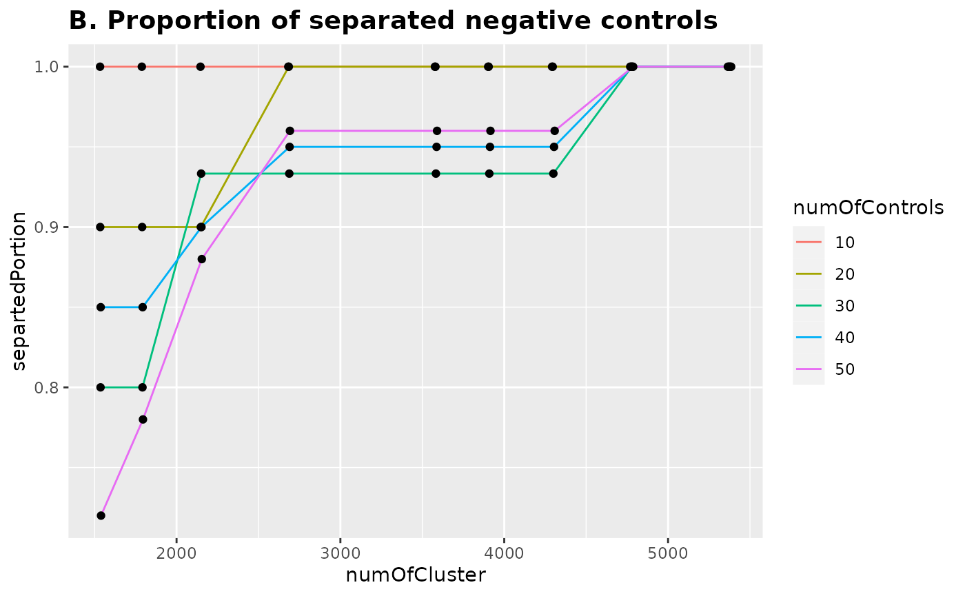
## agg_png 
##       2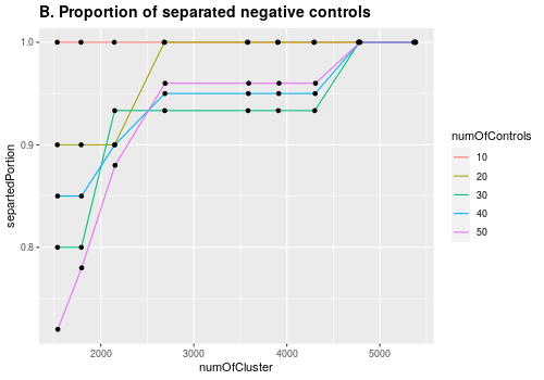

Session Info

sessionInfo()
## R version 4.1.2 (2021-11-01)
## Platform: x86_64-pc-linux-gnu (64-bit)
## Running under: Ubuntu 20.04.3 LTS
## 
## Matrix products: default
## BLAS/LAPACK: /usr/lib/x86_64-linux-gnu/openblas-pthread/libopenblasp-r0.3.8.so
## 
## locale:
##  [1] LC_CTYPE=en_US.UTF-8       LC_NUMERIC=C              
##  [3] LC_TIME=en_US.UTF-8        LC_COLLATE=en_US.UTF-8    
##  [5] LC_MONETARY=en_US.UTF-8    LC_MESSAGES=en_US.UTF-8   
##  [7] LC_PAPER=en_US.UTF-8       LC_NAME=C                 
##  [9] LC_ADDRESS=C               LC_TELEPHONE=C            
## [11] LC_MEASUREMENT=en_US.UTF-8 LC_IDENTIFICATION=C       
## 
## attached base packages:
## [1] stats     graphics  grDevices utils     datasets  methods   base     
## 
## other attached packages:
## [1] ggplot2_3.3.5    dplyr_1.0.8      BiocStyle_2.22.0
## 
## loaded via a namespace (and not attached):
##  [1] ggrepel_0.9.1         Rcpp_1.0.8.3          circlize_0.4.14      
##  [4] png_0.1-7             assertthat_0.2.1      rprojroot_2.0.2      
##  [7] digest_0.6.29         foreach_1.5.2         utf8_1.2.2           
## [10] R6_2.5.1              stats4_4.1.2          evaluate_0.15        
## [13] highr_0.9             pillar_1.7.0          GlobalOptions_0.1.2  
## [16] rlang_1.0.2           jquerylib_0.1.4       magick_2.7.3         
## [19] S4Vectors_0.32.3      GetoptLong_1.0.5      rmarkdown_2.13       
## [22] pkgdown_2.0.2         labeling_0.4.2        textshaping_0.3.6    
## [25] desc_1.4.1            stringr_1.4.0         munsell_0.5.0        
## [28] compiler_4.1.2        xfun_0.30             pkgconfig_2.0.3      
## [31] systemfonts_1.0.4     BiocGenerics_0.40.0   shape_1.4.6          
## [34] htmltools_0.5.2       tidyselect_1.1.2      tibble_3.1.6         
## [37] bookdown_0.25         IRanges_2.28.0        codetools_0.2-18     
## [40] matrixStats_0.61.0    fansi_1.0.2           crayon_1.5.0         
## [43] withr_2.5.0           grid_4.1.2            jsonlite_1.8.0       
## [46] gtable_0.3.0          lifecycle_1.0.1       factoextra_1.0.7     
## [49] DBI_1.1.2             magrittr_2.0.2        scales_1.1.1         
## [52] cli_3.2.0             stringi_1.7.6         cachem_1.0.6         
## [55] farver_2.1.0          fs_1.5.2              doParallel_1.0.17    
## [58] bslib_0.3.1           ellipsis_0.3.2        ragg_1.2.2           
## [61] generics_0.1.2        vctrs_0.3.8           RColorBrewer_1.1-2   
## [64] rjson_0.2.21          iterators_1.0.14      tools_4.1.2          
## [67] glue_1.6.2            purrr_0.3.4           parallel_4.1.2       
## [70] fastmap_1.1.0         yaml_2.3.5            clue_0.3-60          
## [73] colorspace_2.0-3      cluster_2.1.2         BiocManager_1.30.16  
## [76] ComplexHeatmap_2.10.0 memoise_2.0.1         knitr_1.37           
## [79] sass_0.4.0

Sehyun Oh