GenomicSuperSignature - Quickstart
Sehyun Oh
July 27, 2022
Source:vignettes/Quickstart.Rmd
Quickstart.RmdAbstract
This vigenette demostrates a basic usage of GenomicSuperSignature. More extensive and biology-relavant use cases are available HERE.
Setup
Install and load package
if (!require("BiocManager"))
    install.packages("BiocManager")
BiocManager::install("GenomicSuperSignature")
BiocManager::install("bcellViper")
library(GenomicSuperSignature)
library(bcellViper)
Download RAVmodel
You can download GenomicSuperSignature from Google Cloud bucket using
GenomicSuperSignature::getModel function. Currently
available models are built from top 20 PCs of 536 studies (containing
44,890 samples) containing 13,934 common genes from each of 536 study’s
top 90% varying genes based on their study-level standard deviation.
There are two versions of this RAVmodel annotated with different gene
sets for GSEA - MSigDB C2 (C2) and three priors from PLIER
package (PLIERpriors).
The demo in this vignette is based on human B-cell expression data,
so we are using the PLIERpriors model annotated with
blood-associated gene sets.
Note that the first interactive run of this code, you will be asked
to allow R to create a cache directory. The model file will be stored
there and subsequent calls to getModel will read from the
cache.
RAVmodel <- getModel("PLIERpriors", load=TRUE)
#> [1] "downloading"
RAVmodel
#> class: PCAGenomicSignatures
#> dim: 13934 4764
#> metadata(8): cluster size ... version geneSets
#> assays(1): RAVindex
#> rownames(13934): CASKIN1 DDX3Y ... CTC-457E21.9 AC007966.1
#> rowData names(0):
#> colnames(4764): RAV1 RAV2 ... RAV4763 RAV4764
#> colData names(4): RAV studies silhouetteWidth gsea
#> trainingData(2): PCAsummary MeSH
#> trainingData names(536): DRP000987 SRP059172 ... SRP164913 SRP188526

version(RAVmodel)
#> [1] "1.1.1"
Example dataset
The human B-cell dataset (Gene Expression Omnibus series GSE2350) consists of 211 normal and tumor human B-cell phenotypes. This dataset was generated on Affymatrix HG-U95Av2 arrays and stored in an ExpressionSet object with 6,249 features x 211 samples.
data(bcellViper)
dset
#> ExpressionSet (storageMode: lockedEnvironment)
#> assayData: 6249 features, 211 samples
#>   element names: exprs
#> protocolData: none
#> phenoData
#>   sampleNames: GSM44075 GSM44078 ... GSM44302 (211 total)
#>   varLabels: sampleID description detailed_description
#>   varMetadata: labelDescription
#> featureData: none
#> experimentData: use 'experimentData(object)'
#> Annotation:
You can provide your own expression dataset in any of these formats: simple matrix, ExpressionSet, or SummarizedExperiment. Just make sure that genes are in a ‘symbol’ format.
Which RAV best represents the dataset?
validate function calculates validation score, which
provides a quantitative representation of the relevance between a new
dataset and RAV. RAVs that give the validation score is called
validated RAV. The validation results can be displayed
in different ways for more intuitive interpretation.
val_all <- validate(dset, RAVmodel)
head(val_all)
#>          score PC          sw cl_size cl_num
#> RAV1 0.2249382  2 -0.05470163       6      1
#> RAV2 0.3899341  2  0.06426256      21      2
#> RAV3 0.1887409  2 -0.01800335       4      3
#> RAV4 0.2309703  6 -0.04005584       7      4
#> RAV5 0.2017431  2  0.05786189       3      5
#> RAV6 0.1903602  8 -0.02520973       3      6
HeatmapTable
heatmapTable takes validation results as its input and
displays them into a two panel table: the top panel shows the average
silhouette width (avg.sw) and the bottom panel displays the validation
score.
heatmapTable can display different subsets of the
validation output. For example, if you specify scoreCutoff,
any validation result above that score will be shown. If you specify the
number (n) of top validation results through num.out, the
output will be a n-columned heatmap table. You can also use the average
silhouette width (swCutoff), the size of cluster
(clsizecutoff), one of the top 8 PCs from the dataset
(whichPC).
Here, we print out top 5 validated RAVs with average silhouette width above 0.
heatmapTable(val_all, RAVmodel, num.out = 5, swCutoff = 0)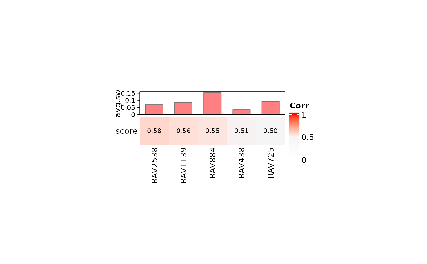
Interactive Graph
Under the default condition, plotValidate plots
validation results of all non single-element RAVs in one graph, where
x-axis represents average silhouette width of the RAVs (a quality
control measure of RAVs) and y-axis represents validation score. We
recommend users to focus on RAVs with higher validation score and use
average silhouette width as a secondary criteria.
plotValidate(val_all, interactive = FALSE)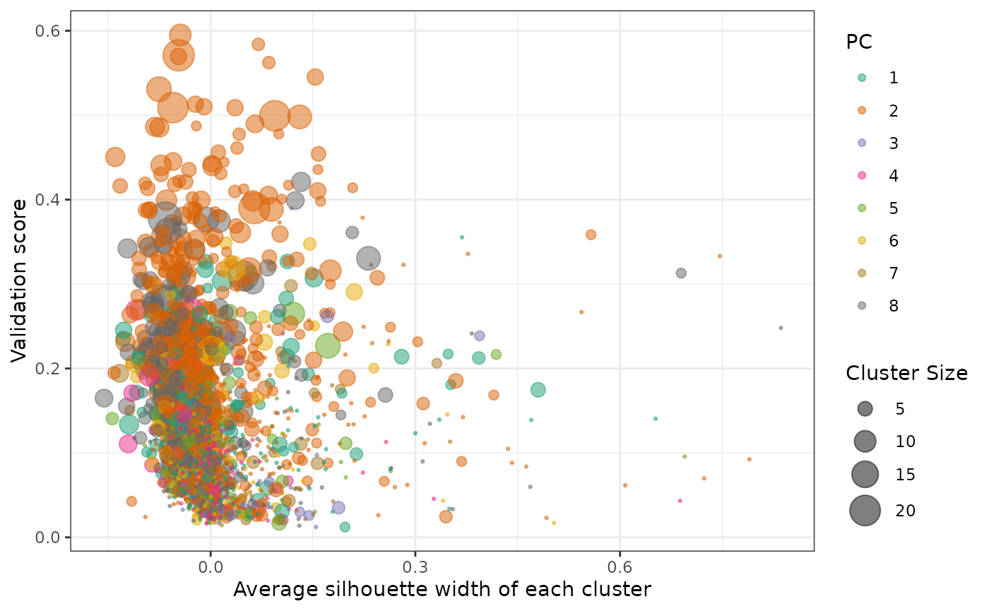
Note that interactive = TRUE will result in a zoomable,
interactive plot that included tooltips.
You can hover each data point for more information:
-
sw : the average silhouette width of the
cluster
-
score : the top validation score between 8 PCs of
the dataset and RAVs
-
cl_size : the size of RAVs, represented by the dot
size
-
cl_num : the RAV number. You need this index to
find more information about the RAV.
- PC : test dataset’s PC number that validates the given RAV. Because we used top 8 PCs of the test dataset for validation, there are 8 categories.
If you double-click the PC legend on the right, you will enter an individual display mode where you can add an additional group of data point by single-click.
What kinds of information can you access through RAV?
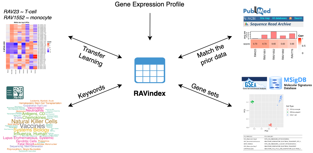
GenomicSuperSignature connects different public databases and prior information through RAVmodel, creating the knowledge graph illustrated below. Through RAVs, you can access and explore the knowledge graph from multiple entry points such as gene expression profiles, publications, study metadata, keywords in MeSH terms and gene sets.
MeSH terms in wordcloud
You can draw a wordcloud with the enriched MeSH terms of RAVs. Based
on the heatmap table above, three RAVs (2538, 1139, and 884) show the
high validation scores with the positive average silhouette widths, so
we draw wordclouds of those RAVs using drawWordcloud
function. You need to provide RAVmodel and the index of the RAV you are
interested in.
Index of validated RAVs can be easily collected using
validatedSingatures function, which outputs the validated
index based on num.out, PC from dataset
(whichPC) or any *Cutoff arguments in the same
way as heatmapTable. Here, we choose the top 3 RAVs with
the average silhouette width above 0, which will returns RAV2538,
RAV1139, and RAV884 as we discussed above.
validated_ind <- validatedSignatures(val_all, RAVmodel, num.out = 3,
                                     swCutoff = 0, indexOnly = TRUE)
validated_ind
#> [1] 2538 1139  884
And we plot the wordcloud of those three RAVs.
set.seed(1) # only if you want to reproduce identical display of the same words
drawWordcloud(RAVmodel, validated_ind[1])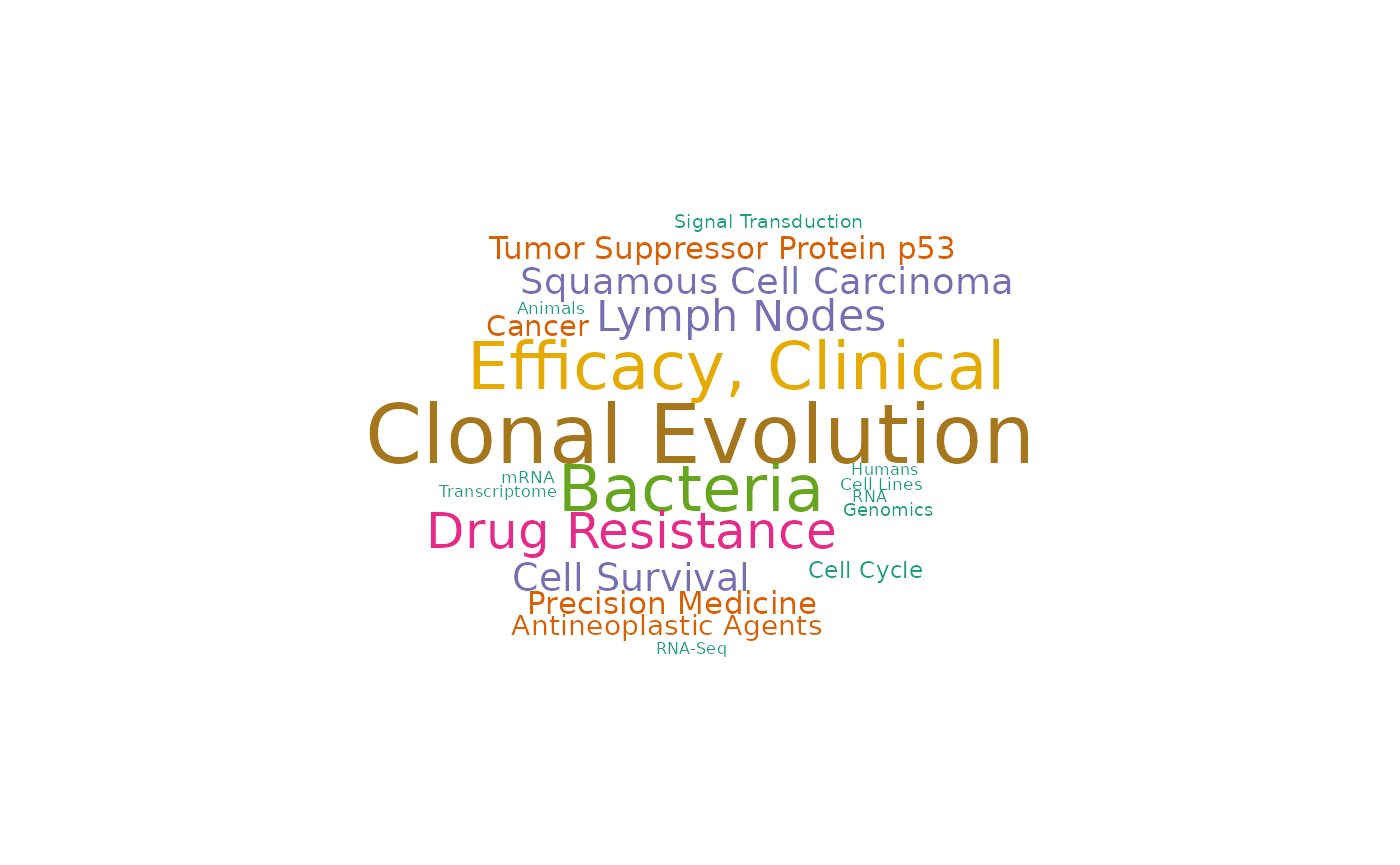
drawWordcloud(RAVmodel, validated_ind[2])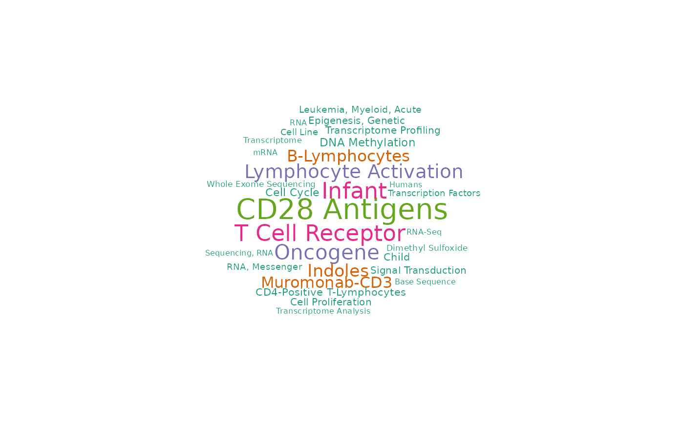
drawWordcloud(RAVmodel, validated_ind[3])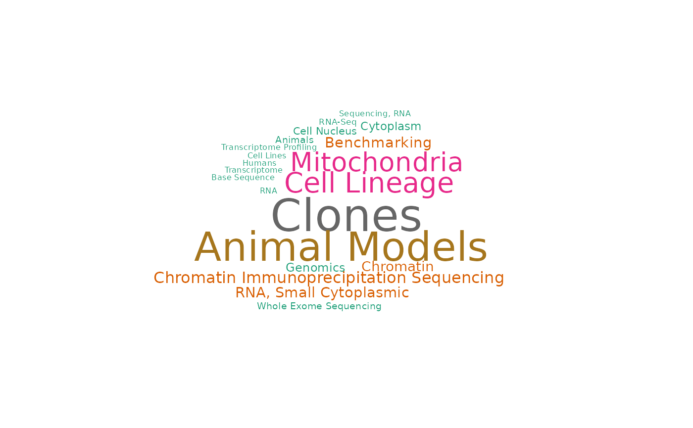
GSEA
Associated gene sets of validated RAV
You can directly access the GSEA outputs for each RAV using
annotateRAV function. Based on the wordclouds, RAV1139
seems to be associated with B-cell.
annotateRAV(RAVmodel, validated_ind[2]) # RAV1139
#>                                        Description       NES pvalue
#> 1                                        DMAP_ERY3 -2.179082  1e-10
#> 2                          KEGG_ALZHEIMERS_DISEASE -2.443701  1e-10
#> 3 REACTOME_POST_TRANSLATIONAL_PROTEIN_MODIFICATION -2.458995  1e-10
#> 4                               REACTOME_APOPTOSIS -2.645437  1e-10
#> 5                         KEGG_HUNTINGTONS_DISEASE -2.670108  1e-10
#>        qvalues
#> 1 6.390977e-10
#> 2 6.390977e-10
#> 3 6.390977e-10
#> 4 6.390977e-10
#> 5 6.390977e-10
If you want to check the enriched pathways for multiple RAVs, use
subsetEnrichedPathways function instead.
subsetEnrichedPathways(RAVmodel, validated_ind[2], include_nes = TRUE)
#> DataFrame with 10 rows and 2 columns
#>          RAV1139.Description RAV1139.NES
#>                  <character>   <numeric>
#> Up_1               DMAP_ERY3    -2.17908
#> Up_2  KEGG_ALZHEIMERS_DISE..    -2.44370
#> Up_3  REACTOME_POST_TRANSL..    -2.45899
#> Up_4      REACTOME_APOPTOSIS    -2.64544
#> Up_5  KEGG_HUNTINGTONS_DIS..    -2.67011
#> Up_6  REACTOME_MRNA_PROCES..    -2.67431
#> Up_7  REACTOME_HOST_INTERA..    -2.69593
#> Up_8         PID_E2F_PATHWAY    -2.74887
#> Up_9  KEGG_PYRIMIDINE_META..    -2.75404
#> Up_10 REACTOME_CDK_MEDIATE..    -2.75535

subsetEnrichedPathways(RAVmodel, validated_ind, include_nes = TRUE)
#> DataFrame with 10 rows and 6 columns
#>          RAV2538.Description RAV2538.NES    RAV1139.Description RAV1139.NES
#>                  <character>   <numeric>            <character>   <numeric>
#> Up_1     REACTOME_CELL_CYCLE     3.25799              DMAP_ERY3    -2.17908
#> Up_2  REACTOME_CELL_CYCLE_..     3.22323 KEGG_ALZHEIMERS_DISE..    -2.44370
#> Up_3  REACTOME_DNA_REPLICA..     3.18974 REACTOME_POST_TRANSL..    -2.45899
#> Up_4  REACTOME_MITOTIC_M_M..     3.10711     REACTOME_APOPTOSIS    -2.64544
#> Up_5  REACTOME_MITOTIC_PRO..     2.91384 KEGG_HUNTINGTONS_DIS..    -2.67011
#> Up_6         KEGG_CELL_CYCLE     2.86725 REACTOME_MRNA_PROCES..    -2.67431
#> Up_7  REACTOME_CHROMOSOME_..     2.85931 REACTOME_HOST_INTERA..    -2.69593
#> Up_8        REACTOME_S_PHASE     2.85345        PID_E2F_PATHWAY    -2.74887
#> Up_9  REACTOME_MITOTIC_G1_..     2.83497 KEGG_PYRIMIDINE_META..    -2.75404
#> Up_10 REACTOME_CELL_CYCLE_..     2.80616 REACTOME_CDK_MEDIATE..    -2.75535
#>           RAV884.Description RAV884.NES
#>                  <character>  <numeric>
#> Up_1               DMAP_ERY3   -1.43162
#> Up_2  REACTOME_METABOLISM_..   -1.54368
#> Up_3  KEGG_ALZHEIMERS_DISE..   -1.62716
#> Up_4  KEGG_HUNTINGTONS_DIS..   -1.65062
#> Up_5         KEGG_CELL_CYCLE   -1.65473
#> Up_6  REACTOME_MITOTIC_G1_..   -1.67482
#> Up_7  REACTOME_METABOLISM_..   -1.68713
#> Up_8     REACTOME_CELL_CYCLE   -1.69922
#> Up_9  REACTOME_CELL_CYCLE_..   -1.72169
#> Up_10 REACTOME_DNA_REPLICA..   -1.76756
Search enriched pathways through keyword
You can also find the RAVs annotated with the keyword-containing
pathways using findSignature function. Without the
k argument, this function outputs a data frame with two
columns: the number of RAVs (Freq column) with the
different numbers of keyword-containing, enriched pathways
(# of keyword-containing pathways column).
Here, we used the keyword, “Bcell”.
findSignature(RAVmodel, "Bcell")
#>   # of keyword-containing pathways Freq
#> 1                                0 4678
#> 2                                1   46
#> 3                                2   15
#> 4                                3   16
#> 5                                4    6
#> 6                                5    3
There are two RAVs with five keyword-containing pathways (row 6). We can check which RAVs they are.
findSignature(RAVmodel, "Bcell", k = 5)
#> [1]  695  953 1994
Enriched pathways are ordered by NES and you can check the rank of
any keyword- containing pathways using
findKeywordInRAV.
findKeywordInRAV(RAVmodel, "Bcell", ind = 695)
#> [1] "1|2|3|4|5|6|8 (out of 9)"
You can check all enriched pathways of RAV using
subsetEnrichedPathways function. If both=TRUE,
both the top and bottom enriched pathways will be printed.
## Chosen based on validation/MeSH terms
subsetEnrichedPathways(RAVmodel, ind = validated_ind[2], n = 3, both = TRUE)
#> DataFrame with 6 rows and 1 column
#>           RAV1139.Description
#>                   <character>
#> Up_1                DMAP_ERY3
#> Up_2   KEGG_ALZHEIMERS_DISE..
#> Up_3   REACTOME_POST_TRANSL..
#> Down_1 REACTOME_CELL_CYCLE_..
#> Down_2 REACTOME_DNA_REPLICA..
#> Down_3    REACTOME_CELL_CYCLE

## Chosen based on enriched pathways
subsetEnrichedPathways(RAVmodel, ind = 695, n = 3, both = TRUE)
#> DataFrame with 6 rows and 1 column
#>            RAV695.Description
#>                   <character>
#> Up_1   IRIS_Bcell-Memory_Ig..
#> Up_2             DMAP_BCELLA3
#> Up_3         IRIS_Bcell-naive
#> Down_1     SVM B cells memory
#> Down_2           DMAP_BCELLA1
#> Down_3 IRIS_PlasmaCell-From..
subsetEnrichedPathways(RAVmodel, ind = 953, n = 3, both = TRUE)
#> DataFrame with 6 rows and 1 column
#>            RAV953.Description
#>                   <character>
#> Up_1   IRIS_Bcell-Memory_Ig..
#> Up_2    IRIS_Bcell-Memory_IgM
#> Up_3         IRIS_Bcell-naive
#> Down_1     IRIS_Monocyte-Day0
#> Down_2 IRIS_DendriticCell-L..
#> Down_3     IRIS_Monocyte-Day1
subsetEnrichedPathways(RAVmodel, ind = 1994, n = 3, both = TRUE)
#> DataFrame with 6 rows and 1 column
#>           RAV1994.Description
#>                   <character>
#> Up_1   SVM T cells CD4 memo..
#> Up_2             DMAP_TCELLA6
#> Up_3             DMAP_TCELLA8
#> Down_1       IRIS_Bcell-naive
#> Down_2  IRIS_Bcell-Memory_IgM
#> Down_3 IRIS_Bcell-Memory_Ig..
Related prior studies
You can find the prior studies related to a given RAV using
findStudiesInCluster function.
findStudiesInCluster(RAVmodel, validated_ind[2])
#>   studyName PC Variance explained (%)
#> 1 SRP028567  2                  14.76
#> 2 SRP059057  3                   7.45
#> 3 SRP095405  1                  37.27
#> 4 SRP144647  1                  32.82
You can easily extract the study name with the
studyTitle=TRUE parameter.
findStudiesInCluster(RAVmodel, validated_ind[2], studyTitle = TRUE)
#>   studyName PC Variance explained (%)
#> 1 SRP028567  2                  14.76
#> 2 SRP059057  3                   7.45
#> 3 SRP095405  1                  37.27
#> 4 SRP144647  1                  32.82
#>                                                                                                                                              title
#> 1                                                                       RNA-Seq analysis of primary AML specimens exposed to AhR modulating agents
#> 2                                                              Transcriptome analysis of CD4+ T cells reveals imprint of BACH2 and IFN? regulation
#> 3 Identification of genes induced by NOTCH1 in a chronic lymphocytic leukaemia (CLL) cell line and tracking of these genes in primary CLL patients
#> 4                                         Transcriptomes from naïve CD4+ T-cells from infants and children with and without food allergy [RNA-seq]
Session Info
sessionInfo()
#> R version 4.2.0 (2022-04-22)
#> Platform: x86_64-pc-linux-gnu (64-bit)
#> Running under: Ubuntu 20.04.4 LTS
#>
#> Matrix products: default
#> BLAS:   /usr/lib/x86_64-linux-gnu/openblas-pthread/libblas.so.3
#> LAPACK: /usr/lib/x86_64-linux-gnu/openblas-pthread/liblapack.so.3
#>
#> locale:
#>  [1] LC_CTYPE=en_US.UTF-8       LC_NUMERIC=C
#>  [3] LC_TIME=en_US.UTF-8        LC_COLLATE=en_US.UTF-8
#>  [5] LC_MONETARY=en_US.UTF-8    LC_MESSAGES=en_US.UTF-8
#>  [7] LC_PAPER=en_US.UTF-8       LC_NAME=C
#>  [9] LC_ADDRESS=C               LC_TELEPHONE=C
#> [11] LC_MEASUREMENT=en_US.UTF-8 LC_IDENTIFICATION=C
#>
#> attached base packages:
#> [1] stats4    stats     graphics  grDevices utils     datasets  methods
#> [8] base
#>
#> other attached packages:
#>  [1] bcellViper_1.32.0           GenomicSuperSignature_1.4.0
#>  [3] SummarizedExperiment_1.26.1 Biobase_2.56.0
#>  [5] GenomicRanges_1.48.0        GenomeInfoDb_1.32.2
#>  [7] IRanges_2.30.0              S4Vectors_0.34.0
#>  [9] BiocGenerics_0.42.0         MatrixGenerics_1.8.1
#> [11] matrixStats_0.62.0          BiocStyle_2.24.0
#>
#> loaded via a namespace (and not attached):
#>   [1] colorspace_2.0-3       ggsignif_0.6.3         rjson_0.2.21
#>   [4] ellipsis_0.3.2         rprojroot_2.0.3        circlize_0.4.15
#>   [7] XVector_0.36.0         GlobalOptions_0.1.2    fs_1.5.2
#>  [10] clue_0.3-61            ggpubr_0.4.0           farver_2.1.1
#>  [13] bit64_4.0.5            fansi_1.0.3            codetools_0.2-18
#>  [16] doParallel_1.0.17      cachem_1.0.6           knitr_1.39
#>  [19] jsonlite_1.8.0         broom_1.0.0            cluster_2.1.3
#>  [22] dbplyr_2.2.1           png_0.1-7              BiocManager_1.30.18
#>  [25] readr_2.1.2            compiler_4.2.0         httr_1.4.3
#>  [28] backports_1.4.1        assertthat_0.2.1       Matrix_1.4-1
#>  [31] fastmap_1.1.0          cli_3.3.0              htmltools_0.5.3
#>  [34] tools_4.2.0            gtable_0.3.0           glue_1.6.2
#>  [37] GenomeInfoDbData_1.2.8 dplyr_1.0.9            rappdirs_0.3.3
#>  [40] Rcpp_1.0.9             carData_3.0-5          jquerylib_0.1.4
#>  [43] pkgdown_2.0.6          vctrs_0.4.1            iterators_1.0.14
#>  [46] xfun_0.31              stringr_1.4.0          lifecycle_1.0.1
#>  [49] rstatix_0.7.0          zlibbioc_1.42.0        scales_1.2.0
#>  [52] ragg_1.2.2             hms_1.1.1              parallel_4.2.0
#>  [55] RColorBrewer_1.1-3     ComplexHeatmap_2.12.0  yaml_2.3.5
#>  [58] curl_4.3.2             memoise_2.0.1          ggplot2_3.3.6
#>  [61] sass_0.4.2             stringi_1.7.8          RSQLite_2.2.15
#>  [64] highr_0.9              desc_1.4.1             foreach_1.5.2
#>  [67] filelock_1.0.2         shape_1.4.6            rlang_1.0.4
#>  [70] pkgconfig_2.0.3        systemfonts_1.0.4      bitops_1.0-7
#>  [73] evaluate_0.15          lattice_0.20-45        purrr_0.3.4
#>  [76] labeling_0.4.2         bit_4.0.4              tidyselect_1.1.2
#>  [79] magrittr_2.0.3         bookdown_0.27          R6_2.5.1
#>  [82] magick_2.7.3           generics_0.1.3         DelayedArray_0.22.0
#>  [85] DBI_1.1.3              pillar_1.8.0           abind_1.4-5
#>  [88] RCurl_1.98-1.7         tibble_3.1.8           crayon_1.5.1
#>  [91] car_3.1-0              wordcloud_2.6          utf8_1.2.2
#>  [94] BiocFileCache_2.4.0    tzdb_0.3.0             rmarkdown_2.14
#>  [97] GetoptLong_1.0.5       grid_4.2.0             blob_1.2.3
#> [100] digest_0.6.29          tidyr_1.2.0            textshaping_0.3.6
#> [103] munsell_0.5.0          bslib_0.4.0