download.file(url = "https://ndownloader.figshare.com/files/2292169",
destfile = "data/portal_data_joined.csv")Session 3_2. Starting with Data
Questions
- How can I read a complete csv file into R?
- What is a data.frame?
- How can I get basic summary information about my dataset?
- How can I change the way R treats strings in my dataset?
- Why would I want strings to be treated differently?
Learning Objectives
- Describe what a data frame is
- Load external data from a .csv file into a data frame
- Summarize the contents of a data frame
- Subset values from data frames
- Describe the difference between a factor and a string
- Change how character strings are handled in a data frame
Loading the data
We are investigating the animal species diversity and weights found within plots at our study site. The dataset is stored as a comma separated value (CSV) file. Each row holds information for a single animal, and the columns represent:
| Column | Description |
|---|---|
| record_id | Unique id for the observation |
| month | month of observation |
| day | day of observation |
| year | year of observation |
| plot_id | ID of a particular experimental plot of land |
| species_id | 2-letter code |
| sex | sex of animal (“M”, “F”) |
| hindfoot_length | length of the hindfoot in mm |
| weight | weight of the animal in grams |
| genus | genus of animal |
| species | species of animal |
| taxon | e.g. Rodent, Reptile, Bird, Rabbit |
| plot_type | type of plot |
Downloading the data
We created the folder that will store the downloaded data (data) in the previous session. We are going to use the R function download.file() to download the CSV file that contains the survey data from Figshare, and we will use read_csv() to load the content of the CSV file into R.
Reading the data into R
The file has now been downloaded to the destination you specified, but R has not yet loaded the data from the file into memory. To do this, we can use the read_csv() function from the tidyverse package.
To install the tidyverse package, we can type install.packages("tidyverse") straight into the console. You don’t need to re-install packages every time you need them. To load the installed package:
Use read_csv() to read the data into a data frame.
surveys <- read_csv("data/portal_data_joined.csv")Rows: 34786 Columns: 13
── Column specification ────────────────────────────────────────────────────────
Delimiter: ","
chr (6): species_id, sex, genus, species, taxa, plot_type
dbl (7): record_id, month, day, year, plot_id, hindfoot_length, weight
ℹ Use `spec()` to retrieve the full column specification for this data.
ℹ Specify the column types or set `show_col_types = FALSE` to quiet this message.When you execute read_csv on a data file, it looks through the first 1000 rows of each column and guesses its data type. For example, in this dataset, read_csv() reads weight as col_double (a numeric data type), and species as col_character. You have the option to specify the data type for a column manually by using the col_types argument in read_csv.
read_csv() assumes that fields are delineated by commas. However, in several countries, the comma is used as a decimal separator and the semicolon (;) is used as a field delineator. If you want to read in this type of files in R, you can use the read_csv2() function. It behaves like read_csv() but uses different parameters for the decimal and the field separators. There is also the read_tsv() for tab separated data files and read_delim() for less common formats. Check out the help for read_csv() by typing ?read_csv to learn more.
Also, check this for importing data from text/csv files, excel files, and SPSS, SAS and Stata files into RStudio IDE.
We can see the contents of the first few lines of the data by typing its name: surveys. We can also extract the first few lines of this data using the function head():
head(surveys)# A tibble: 6 × 13
record_id month day year plot_id species_id sex hindfoot_length weight
<dbl> <dbl> <dbl> <dbl> <dbl> <chr> <chr> <dbl> <dbl>
1 1 7 16 1977 2 NL M 32 NA
2 72 8 19 1977 2 NL M 31 NA
3 224 9 13 1977 2 NL <NA> NA NA
4 266 10 16 1977 2 NL <NA> NA NA
5 349 11 12 1977 2 NL <NA> NA NA
6 363 11 12 1977 2 NL <NA> NA NA
# ℹ 4 more variables: genus <chr>, species <chr>, taxa <chr>, plot_type <chr>You can assign the first 100 rows of surveys to an object using surveys_sample <- head(surveys, 100). This can be useful if you want to try out complex computations on a subset of your data before you apply them to the whole data set.
There is a similar function that lets you extract the last few lines of the dataset, called tail().
To open the dataset in RStudio’s Data Viewer, use the view() function:
view(surveys)Data frame
What is data frame?
[Reminder from the session2_2] A data frame is the representation of data in the format of a table where the columns are vectors that all have the same length. Because columns are vectors, each column must contain a single type of data (e.g., characters, integers, factors).
When we loaded the data into R, it got stored as an object of class tibble, which is a special kind of data frame (the difference is not important for our purposes, but you can learn more about tibbles here).
Inspecting data frames
Here is a non-exhaustive list of functions to get a sense of the content/structure of the data.
-
Size:
-
dim(surveys)- returns a vector with the number of rows in the first element, and the number of columns as the second element (the dimensions of the object) -
nrow(surveys)- returns the number of rows -
ncol(surveys)- returns the number of columns
-
-
Content:
-
head(surveys)- shows the first 6 rows -
tail(surveys)- shows the last 6 rows
-
-
Names:
-
names(surveys)- returns the column names (synonym ofcolnames()fordata.frameobjects) -
rownames(surveys)- returns the row names
-
-
Summary:
-
str(surveys)- structure of the object and information about the class, length and content of each column -
summary(surveys)- summary statistics for each column
-
Indexing and subsetting data frames
If you want to subset data, you need to specify the “coordinates” that you want from it. Row numbers come first, followed by column numbers. However, note that different ways of specifying these coordinates lead to results with different classes.
# Extract the first row and column from surveys table:
surveys[1, 1]

# First row, sixth column:
surveys[1, 6]

## To select all columns, leave the column index blank
# Select the first row:
surveys[1, ]

# Select the first column
surveys[, 1]

# An even shorter way to select first column across all rows:
surveys[1] # No comma!
: is a special function that creates numeric vectors of integers in increasing or decreasing order.
Subsetting with single square brackets ([]) always returns a data frame. If you want a vector, use double square brackets ([[]])
# To get the first column as a vector:
surveys[[1]]
You can also exclude certain indices of a data frame using the - sign:
surveys[, -1]                 # The whole data frame, except the first column
surveys[-(7:nrow(surveys)), ] # Equivalent to head(surveys)
Data frames can be subset by calling indices (as shown previously), but also by calling their column names directly:
# As before, using single brackets returns a data frame:
surveys["species_id"]
surveys[, "species_id"]

# Double brackets returns a vector:
surveys[["species_id"]]

# We can use the $ operator with column names instead of double brackets
# This returns a vector:
surveys$species_id
Factors
When we did str(surveys) we saw that several of the columns consist of integers. However, the columns such as genus, species, sex, and plot_type are of the class character. Arguably, these columns contain categorical data, that is, they can only take on a limited number of values. R has a special class for working with categorical data, called factor.
Once created, factors can only contain a pre-defined set of values, known as levels. Factors are stored as integers associated with labels and they can be ordered or unordered. While factors look (and often behave) like character vectors, they are actually treated as integer vectors by R.
When importing a data frame with read_csv(), the columns that contain text are not automatically coerced (= converted) into the factor data type, but once we have loaded the data we can do the conversion using the factor() function:
surveys$sex <- factor(surveys$sex)We can see that the conversion has worked by using the summary() function again.
summary(surveys$sex)Levels
By default, R always sorts levels in alphabetical order. For instance, if you have a factor with 2 levels:
R will assign 1 to the level "female" and 2 to the level "male". You can see this by using the function levels() and you can find the number of levels using nlevels():
Sometimes, the order of the factors does not matter, other times you might want to specify the order because it is meaningful (e.g., “low”, “medium”, “high”), it improves your visualization, or it is required by a particular type of analysis. Here, one way to reorder our levels in the sex vector would be:
Renaming factors
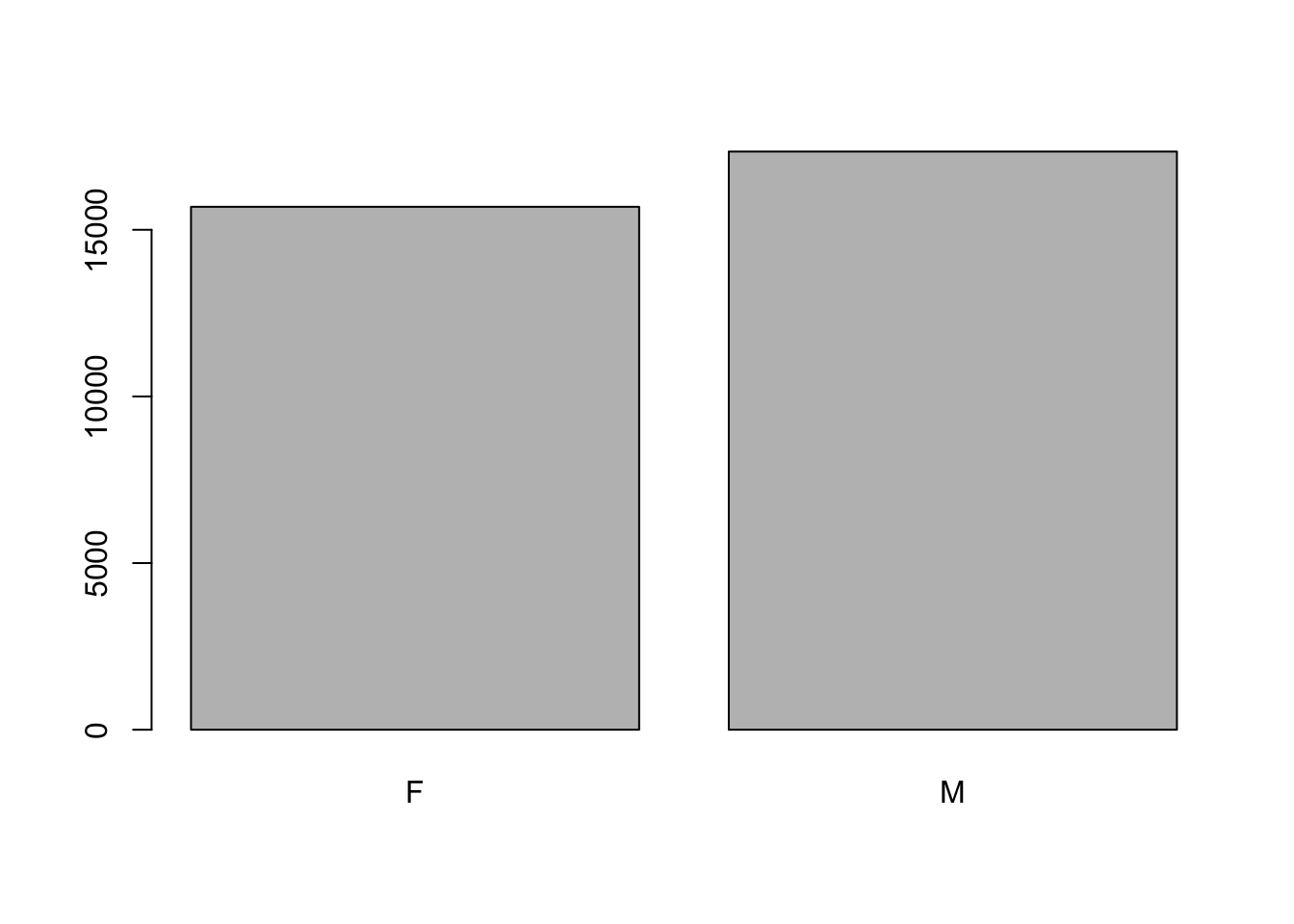
When your data is stored as a factor, you can use the plot() function to get a quick glance at the number of observations represented by each factor level.
## bar plot of the number of females and males
plot(surveys$sex)
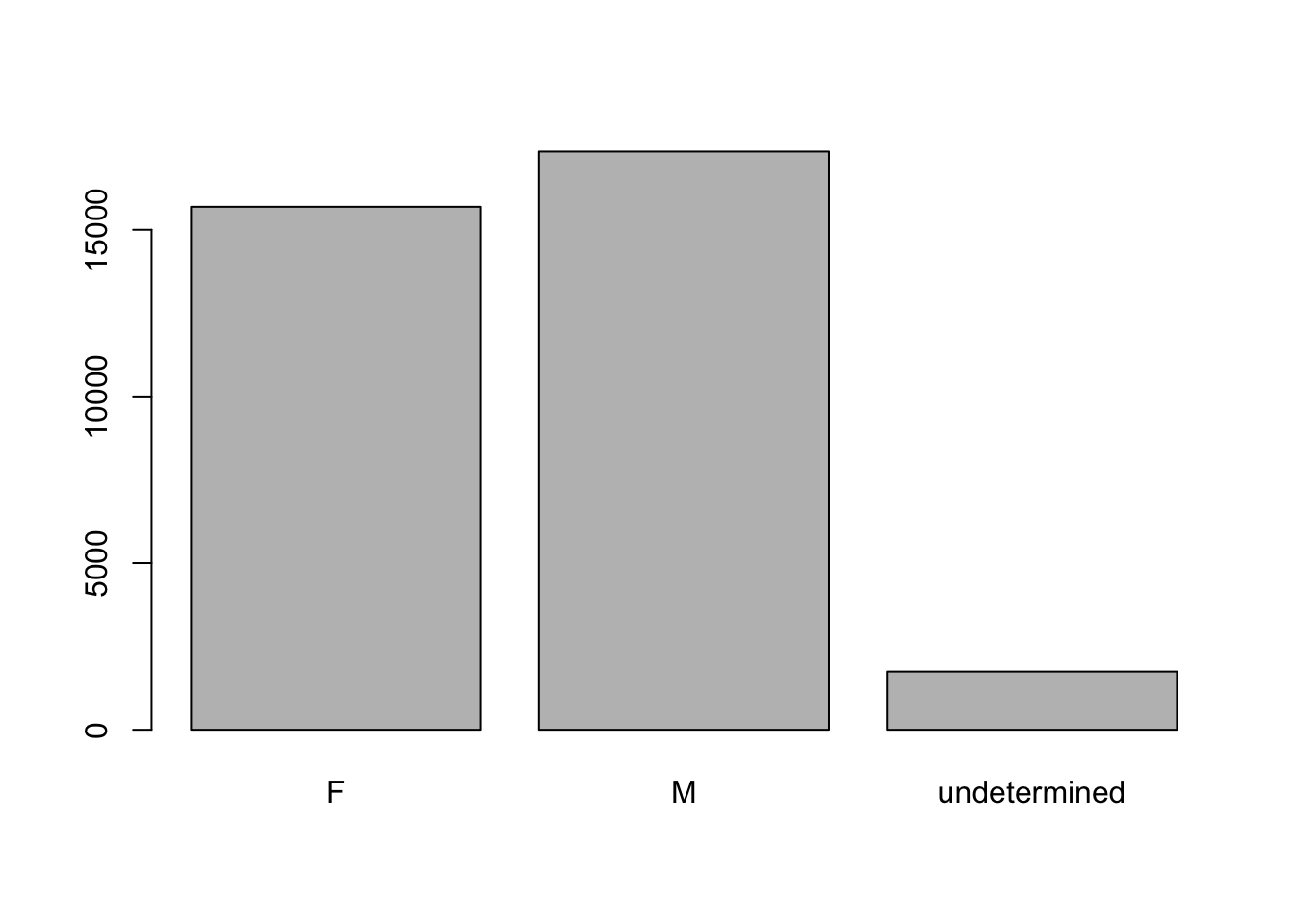
However, this plot misses out some information - as we saw from summary(surveys$sex), there are about 1700 individuals for which the sex information hasn’t been recorded. To show them in the plot, we can turn the missing values into a factor level with the addNA() function. We will also have to give the new factor level a label.
To avoid modifying the working copy of the data frame, we can make a copy of the sex column we want to use:
sex <- surveys$sex
levels(sex)
[1] "F" "M"[1] "F" "M" NA head(sex)[1] M M <NA> <NA> <NA> <NA>
Levels: F M <NA>[1] "F" "M" "undetermined"head(sex)[1] M M undetermined undetermined undetermined
[6] undetermined
Levels: F M undeterminedNow we can plot the data again, using plot(sex).
plot(sex)
Reference
https://datacarpentry.org/r-socialsci/instructor/02-starting-with-data.html
https://datacarpentry.org/R-ecology-lesson/02-starting-with-data.html